Meta-Learning

元学习相关论文。

Model-Agnostic Meta-Learning for Fast Adaptation of Deep Networks

作者将元学习问题形式化后提出了一个模型无关的元学习算法MAML。

问题设置

用 \(f\) 表示一个机器学习中模型，可以将输入分布中的一个观测 \(x\) 映射到输出 \(a\) 。

元学习中，每个任务表示为 \(T={L(x_1,a_1,..,x_H,a_H),q(x_1),q(x_{t+1}|x_t,a_t),H}\)，其中 \(L(x_1,a_1,..,x_H,a_H)\rightarrow \mathbb{R}\) 为损失函数，\(q(x_1)\) 表示初始观测 \(x_1\) 的分布，而 \(q(x_{t+1}|x_t,a_t)\) 表示转移的分布，用于适应不同模型。对于i.i.d的监督学习，\(H=1\)。

考虑学习任务的分布 \(p(T)\) ，元学习要学习的就是该分布。在K样本(K-shot)的学习中，元学习的训练使用分布 \(p(T)\) 中的任务 \(T_i\)，然后用该任务中 \(q_i\) 的K个样本和 \(L_{T_i}\) 进行训练，并用 \(T_i\) 中新的样本进行测试，得到的测试误差用作整个元学习的训练误差。最终使用分布 \(p(T)\) 采样的新任务来测试元学习模型。

MAML算法

算法目标是寻找敏感的模型参数，使得其面对分布 \(p(T)\) 中新的任务时，对参数较小的修改就可以使新任务的模型产生很大的提升。算法对模型没有假设，只假设其可以用一组参数 \(\theta\) 表示，并且其可以使用基于梯度的学习技术来更新。

元学习算法中，每个任务中的模型用 \(f_{\theta}\) 表示，并对于一个新的任务 \(T_i\) ，模型适应后参数记为 \(\theta_i'\) ，其可以通过一次或多次梯度下降得到，每次梯度下降可以表示为：

$$ \theta_i' = \theta - \alpha \nabla_\theta L_{T_i}(f_\theta) $$

其中 \(\alpha\) 为超参数或可以被元学习。

元学习的目标是将模型 \(f_{\theta_i'}\) 的效果最优化：

$$ \min_{\theta}\sum_{T_i \sim p(T)}L_{T_i}(f_{\theta_i'})=\sum_{T_i \sim p(T)}L_{T_i}(f_{\theta - \alpha \nabla_\theta L_{T_i}(f_\theta)}) $$

学习目标最终体现在得到的模型参数\(\theta\)中：

$$ \theta \leftarrow \theta - \beta \nabla_\theta \sum_{T_i \sim p(T)}L_{T_i}(f_{\theta_i'}) $$

MAML对新的任务，使用该参数\(\theta\)经过较少的新任务中的样本训练后，就可以得到很好的效果。

监督学习(回归和分类)

设置\(H=1\)。

对于回归类的任务，使用MSE：

$$ L_{T_i}(f_{\phi})=\sum_{x^{(j)},y^{(j)} \sim T_i}||f_\phi(x^{(j)})-y^{(j)}||^2_2 $$

其中，\(x^{(j)},y^{(j)}\)为任务\(T_i\)的样本对，K样本的回归任务中，每个任务取K个进行训练。

对于离散的分类任务，使用cross entropy：

$$ L_{T_i}(f_{\phi})=\sum_{x^{(j)},y^{(j)} \sim T_i}y^{(j)}log f_\phi(x^{(j)})+(1-y^{(j)})log (1-f_\phi(x^{(j)})) $$

K样本N分类任务的训练中，每一类需要K个样本，每个任务需要NK个数据。

强化学习

每个强化学习任务包含初始状态分布\(q_i(x_1)\) ，一个转移分布 \(q_i(x_{t+1}|x_t,a_t)\) 和由(负的)奖励函数\(R\)定义的损失函数\(L_{T_i}\)。整个任务是一个马尔可夫决策过程，长度为H。学习的模型\(f_\theta\)可以将每一步\(t\in{1,...,H}\)的\(x_t\)状态映射到一个动作\(a_t\)上。形式为：

$$ L_{T_i}(f_\phi)=-\mathbb{E_{x_t,a_t \sim f_\phi,q_{T_i}}}[\sum_{t=1}^{H}R_i(x_t,a_t)] $$

测试结果

HOW TO TRAIN YOUR MAML

MAML的问题

• 训练不稳定性

  训练时很不稳定，依赖于神经网络的架构和外层超参数的设定。 可能导致梯度爆炸或梯度消失。

• 二阶导的成本

  梯度更新需要计算二阶导，非常昂贵，MAML中提出使用一阶近似来加速这个过程，但这样做会对最终泛化误差产生负面的影响。 在不牺牲泛化性能的情况下减少计算时间的方法还没有被提出。

• 批处理归一化(Batch Normalization)统计量累积的缺失

  在原MAML论文中实验里批处理归一化使用方式是有问题的，其没有累积得到的统计量，而是直接将当前统计量用于批处理归一化，这样学习到的偏差需要适应不同的均值和标准偏差，而如果使用的是累积的统计量，那么最终会收敛到某个全局的均值和标准偏差，并且这样做收敛更快、更稳定、泛化性能更好。

• 共享(跨步)批处理归一化偏差

  另一个问题是其批处理归一化偏差并不是在inner-loop中更新的，而在整个base-model迭代中使用了同样的bias，这含蓄地假设了所有的base-model在inner-loop中更新时都一样，即其特征有同样的分布，但这个假设是错误的。在每个inner-loop中，会有新的base-model产生，并且其和之前的模型有足够的不同，从bias的估计上应该被认为是一个新的模型。

• 共享内循环(跨步和跨参数)学习率

  还有个同时影响泛化性能和收敛速度(用训练迭代次数表示)的问题是所有参数和更新都使用同一个共享的学习率。这样需要一个固定的学习率，需要进行多次超参数调整，可能会非常昂贵。 Learning to learn quickly for few shot learning. arXiv preprint arXiv:1707.09835, 2017.的作者提出可以对网络每个参数的学习率进行学习，可以解决上述问题，但也有自己的问题，这样会增加计算和内存空间的成本。

• 固定的外循环学习率

  MAML中作者使用固定学习率的Adam来训练元优化器，使用阶跃函数或余弦函数对学习速率进行退火已被证明是在多种设置下实现先进的泛化性能的关键，因此证明了使用静态学习率有可能降低了MAML的泛化性能和优化速度，并且固定的学习率也意味着须花费更多的时间调整。

MAML++

一个一个解决上述问题。

• 梯度不稳定性 -> 多步损失优化(Multi-Step Loss Optimization, MSL)

  在每个base-model的inner-loop中，对support-set中的每一步都对目标进行更新： $$ \theta = \theta - \beta \nabla_\theta \sum_{b=1}^B \sum_{i=0}^N v_i L_{T_b}(f_{\theta_i^b}) $$ b表示任务，i表示每个任务中第i步，\(v_i\)表示第i步后的权重。 还需要对每步损失的权重进行退火，一开始所有损失贡献相同，但随着训练迭代，我们减少靠前步骤的权重，缓慢增加靠后步骤的权重，这保证随着训练的进行，优化器会更重视最终的步骤从而达到最低可能的损失。

• 二阶导成本 -> 导数退火(Derivative-Order Annealing, DA)

  原MAML算法中需要计算二阶导，其作者提出使用一阶近似来计算，但他是在整个训练过程中都使用一阶近似。MAML++提出，可以在前50个epochs中使用一阶近似，而之后都使用二阶导计算，这样经过经验可以得到前50个epochs可以被极大地加速，并且后面使用二阶导计算可以得到很强的泛化性能。 并且还可以观察到，这样做可以避免梯度爆炸和梯度消失，而全部直接使用二阶导会更加不稳定。说明DA比单独使用标准MAML算法更加稳定，使用一阶近似进行训练相当于标准MAML的一种预训练，让后期MAML对模型的训练更好之外，可以避免标准MAML算法出现梯度衰减、梯度爆炸现象。

• 批处理归一化统计量累积的缺失 -> 每步批处理归一化处理统计量(Per-Step Batch Normalization Running Statistics, BNRS)

  MAML++提出在每步中收集统计量，需要在网络的每一批归一化层都实例化N组running均值和标准偏差，然后随着优化的每一步分别更新这些统计量。

• 共享(跨步)批处理归一化偏差 -> 每步的批处理归一化权重和偏差(Per-Step Batch Normalization Weights and Biases, BNWB)

  MAML++提出在inner-loop更新过程中每步都学习一组偏差。这样做意味着Batch Normalization将学习特定于在每个集合处看到的特征分布的偏差，这将提高收敛速度，稳定性和泛化性能。

• 共享内循环(跨步和跨参数)学习率 -> 每层每步的学习率和梯度方向的学习(Learning Per-Layer Per-Step Learning Rates and Gradient Directions, LSLR)

  之前提到，Learning to learn quickly for few shot learning. arXiv preprint arXiv:1707.09835, 2017.的作者提出可以对网络每个参数的学习率进行学习，可以解决上述问题，但也有自己的问题，这样会增加计算和内存空间的成本。 MAML++提出对网络中每一层学习一个学习率和一个搜索方向。

• 固定的外循环学习率 -> 元优化器学习率的余弦退火(Cosine Annealing of Meta-Optimizer Learning Rate, CA)

  原MAML模型采用固定的外循环学习率，MAML++提出对元学习优化器(外循环)学习率使用余弦退火。

实验结果

RAPID LEARNING OR FEATURE REUSE? TOWARDS UNDERSTANDING THE EFFECTIVENESS OF MAML

文章目的是探讨MAML有效的原因是可以快速学习还是特征重复利用，前者模型在遇到新的任务时会进行大量、有效的修改，而后者是说模型在训练之后已经包含了相关任务高质量的特征。

文章直接给出结论：MAML有效的原因是特征重复利用（feature reuse），通过layer freezing experiments和分析MAML模型latent representations来证明结论，并在结论上提出MAML的简化版本ANIL。

FREEZING LAYER REPRESENTATIONS

作者提出模型的网络需要分为两个部分：head和body，head指网络最后一层，body指前面其余的层。

在每个few-shot任务中，网络最后一层也就是head需要将神经元和类别对应起来，所以不同的任务inner-loop训练后head层会有较大不同，所以只需要主要关注body层的表现。

layer freezing experiments指在测试时禁止网络的body层的一个连续子集的参数更新，来对比这些结果，比如：网络一共四层，记为1、2、3、4，最后还有一个head层，实验会进行五次，第一次不禁止更新，第二次禁止第1层更新，第三次禁止第1、2层更新，以此类推。

结果显示对参数禁止更新几乎不影响模型的准确率，即使禁止body中的所有层更新参数，模型的表现也没有怎么下降。

REPRESENTATIONAL SIMILARITY EXPERIMENTS

这个实验分析神经网络在每个任务的inner loop适应后latent representations有多少改变。

作者使用了CCA相似度和CKA相似度来对网络的每一层在inner loop前后的不同进行测试，CCA提供了一种方法可以比较神经网络中的两个层的表示的相似度(从0到1，分数越接近1越相似)，结果发现网络body的所有层相似度都大于0.9，只有head层小于0.5，也符合之前的想法。

ANIL(Almost No Inner Loop)算法

在ANIL算法中，作者移除了训练和测试时inner loop对网络body层的更新，只保留对head层的更新，其余和MAML算法一样。

由于ANIL算法几乎没有inner loop，其速度有显著提升，并且：

• 模型的表现能够达到MAML的水平，不管是few-shot图像分类还是强化学习场景下。
• ANIL和MAML训练时的loss和acc曲线几乎一致，使用CCA和CKA相似度发现MAML-ANIL表示和MAML-MAML表示以及ANIL-ANIL表示有同样的平均相似度得分，说明两个算法学习的特征是类似的，训练时有没有inner loop更新不会改变学习到的特征种类。

网络head和body的贡献

好的特征已经被学习到的情况下，测试时网络的head有多重要？

NIL(No Inner Loop)算法

在训练之后，好的特征已经被学习到了，探讨此时(测试时)head的重要性。

NIL算法：

• 1.使用ANIL/MAML算法训练一个few-shot模型，作者使用了ANIL。
• 2.测试时，移除训练模型的head，对于每个任务，先将k个有标签的数据(支撑集support set)传入网络的body，得到他们倒数第二层的表示，然后对于一个测试数据，计算他倒数第二层的表示和支撑集的表示的余弦相似度(cosine similarities)，使用这些相似性来加权支撑集的标签。

NIL算法得到的模型性能和ANIL和MAML类似，说明MAML/ANIL训练得到的网络body学习到的特征是最重要的。

网络body的训练方式

NIL又引出一个问题：训练时head和task alignment的重要性。

训练时使用NIL方法，即没有head，得到的模型表现会降低很多，说明训练时head是很重要的。

On First-Order Meta-Learning Algorithms

On the Convergence Theory of Gradient-Based Model-Agnostic Meta-Learning Algorithms

文章研究了MAML和FO-MAML的收敛理论，根据梯度范数分析了它们对于非凸损失函数的计算复杂度和能够达到的准确率级别(level)。

作者提出MAML对于任意的\(\epsilon\)，可以在\(O(1/\epsilon^2)\)次迭代内找到一个\(\epsilon\)-一阶导不动点，每次迭代复杂度为\(O(d^2)\)，\(d\)为问题维数，而FO-MAML将每次迭代的复杂度降低为了\(O(d)\)，但不能保证达到想要的准确率级别。

最后作者提出Hessian-free MAML(HF-MAML)算法，既能保有MAML的所有理论保证，又能降低每次迭代的复杂度为\(O(d)\)。

MAML算法和FO-MAML算法

作者用自己的符号表示了两个算法：

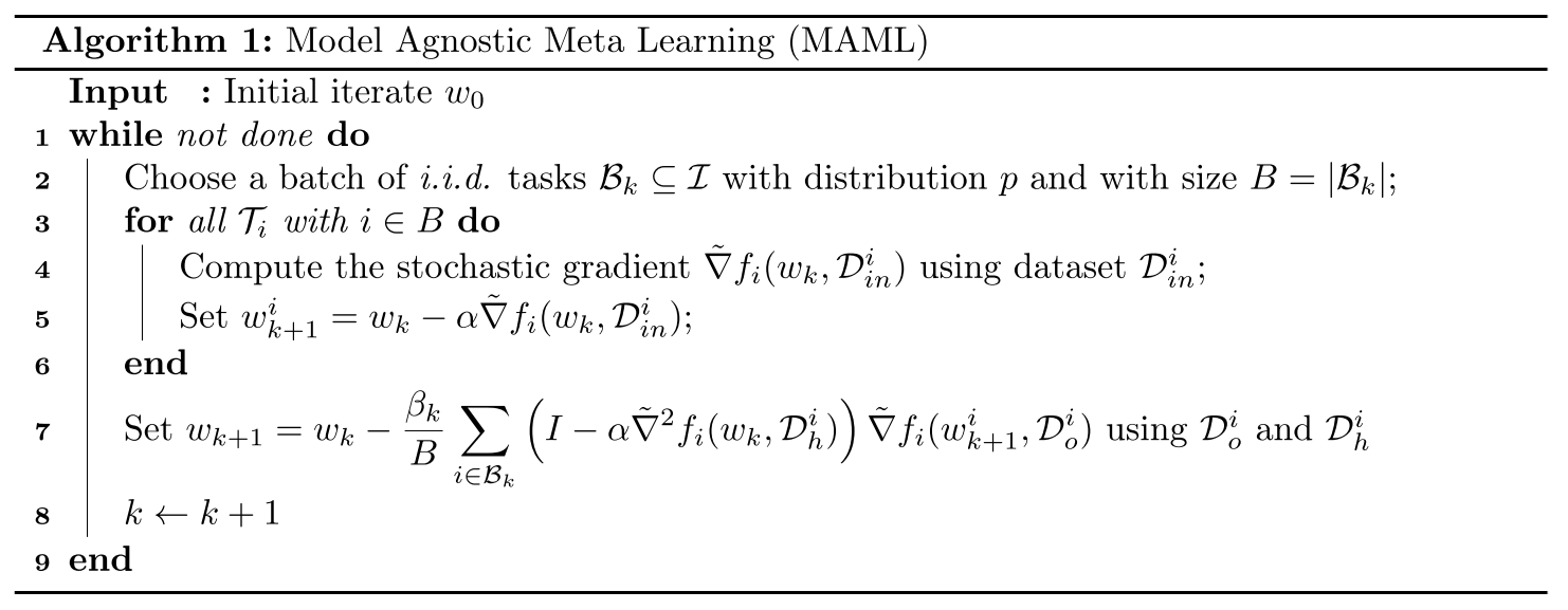
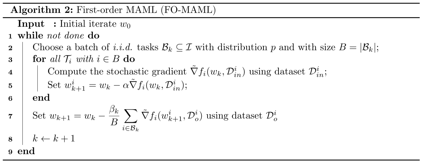
其中MAML算法需要求损失函数的二阶导Hessian矩阵，而FO-MAML将其近似掉了，作者这里设置计算二阶导的数据集\(D_h^i\)和计算一阶导的数据集\(D_o^i\)相互独立，为了使用更小的\(D_h^i\)来减少计算量。

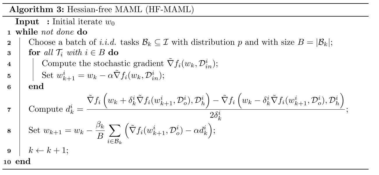
Hessian-free MAML

对于任意函数\(\phi\)，其Hessian矩阵和任意向量\(v\)的乘积可以近似为

$$ \nabla^2\phi(w)v \approx \Bigg[\frac{\nabla\phi(w + \delta v) - \nabla\phi(w - \delta v)}{2\delta}\Bigg] $$

其误差不超过\(\rho\delta||v||^2\)，\(\rho\)为\(\phi\)的Hessian矩阵的利普希茨连续常数。

将其带入之前MAML的更新中得到

$$ d_k^i := \frac{\tilde{\nabla}f_i\Big(w_k+\delta_k^i\tilde{\nabla}f_i(w_k-\alpha \tilde{\nabla}f_i(w_k,D_{in}^i),D_o^i),D_h^i\Big)-f_i\Big(w_k-\delta_k^i\tilde{\nabla}f_i(w_k-\alpha \tilde{\nabla}f_i(w_k,D_{in}^i),D_o^i),D_h^i\Big)}{2\delta_k^i} $$

$$ w_{k+1} = w_k - \beta_k \frac{1}{B} \sum_{i \in B_k} \Big[\tilde{\nabla}f_i(w_k-\alpha \tilde{\nabla}f_i(w_k, D_in^i), D_o^i) - \alpha d_k^i\Big] $$

HF-MAML的算法如下：

理论分析

设\(T = {T_i}_{i \in I} \)表示所有任务的集合，\(p\)表示\(T\)的概率分布，\(T_i\)以\(p_i := p(T_i)\)的概率被抽样，\(T_i\)的损失函数用\(f_i(w):\mathbb{R}^d \rightarrow \mathbb{R}\)表示，定义期望

$$ f(w) := \mathbb{E}_{i \sim p} [f_i(w)] $$

元学习优化问题：

$$ \min_{w \in \mathbb{R}^d} F(w) := \mathbb{E} _ {i \sim p} [F_i(w)] := \mathbb{E} _ {i \sim p} [f_i(w - \alpha \nabla f_i(w))] $$

假设\(F\)为一般的非凸但光滑的函数。

定义1：向量\(w_\epsilon \in \mathbb{R}^d\)被称为上述优化问题的\(\epsilon\)-近似一阶不动点(first order stationary point, FOSP)，如果其满足：

$$ \mathbb{E} [||\nabla F(w_\epsilon)||] \leq \epsilon $$

定义说明一个点\(w_\epsilon\)是一个\(\epsilon\)-FOSP，如果它对全局损失函数\(F\)的梯度模长(gradient norm)的期望小于\(\epsilon\)。

本节的目的是对于MAML、FO-MAML和HF-MAML寻找两个问题的答案：

• 对于任意的\(\epsilon>0\)，可以找到一个\(\epsilon\)-FOSP吗？
• 若可以，需要多少次迭代才能到达该不动点？

假设1：\(F\)有下界，即\(\min_{w \in \mathbb{R}^d} F(w) > -\infty\)。

假设2：对于任意\(i \in I\)，\(f_i\)二次连续可微且\(L_i\)-光滑，即对于任意\(w,u \in \mathbb{R}^d\)，有

$$ ||\nabla f_i(w) - \nabla f_i (u)|| \leq L_i ||w - u|| $$

在二次连续可微的假设下，再假设一阶导\(L_i\)-光滑可以推出：

$$ -L_i I_d \preceq \nabla^2 f_i(w) \preceq L_i I_d, \forall w \in \mathbb{R}^d \ -\frac{L_i}{2} ||w - u||^2 \leq f_i(w) - f_i(u) - \nabla f_i(u)^\top (w-u) \leq \frac{L_i}{2}||w-u||^2, \forall w, u \in \mathbb{R}^d $$

为了简单，此后使用\(L := \max_i L_i\)，可以被看作所有\(i \in I\)的\(\nabla f_i\)利普希茨连续常数。

在MAML的参数更新中出现了\(f_i\)的二阶导，所以需要对目标函数的Hessian矩阵施加一个正则性条件：

假设3：

Meta-Learning with Implicit Gradients

meta-RL

元强化学习相关论文。

Meta-Reinforcement Learning of Structured Exploration Strategies

Prior tasks can be used to inform how exploration in new tasks should be performed.

A meta-RL algorithm that adapts to new tasks by following the policy gradient, while also injecting learned structured stochasticity into a latent space to enable effective exploration.

Effective exploration strategies must select randomly from among the potentially useful behaviors, while avoiding behaviors that are highly unlikely to succeed. MAESN leverages this insight to acquire significantly better exploration strategies by incorporating learned time-correlated noise through its meta-learned latent space, and training both the policy parameters and the latent exploration space explicitly for fast adaptation.

Preliminaries

Model Agnostic Exploration with Structured Noise

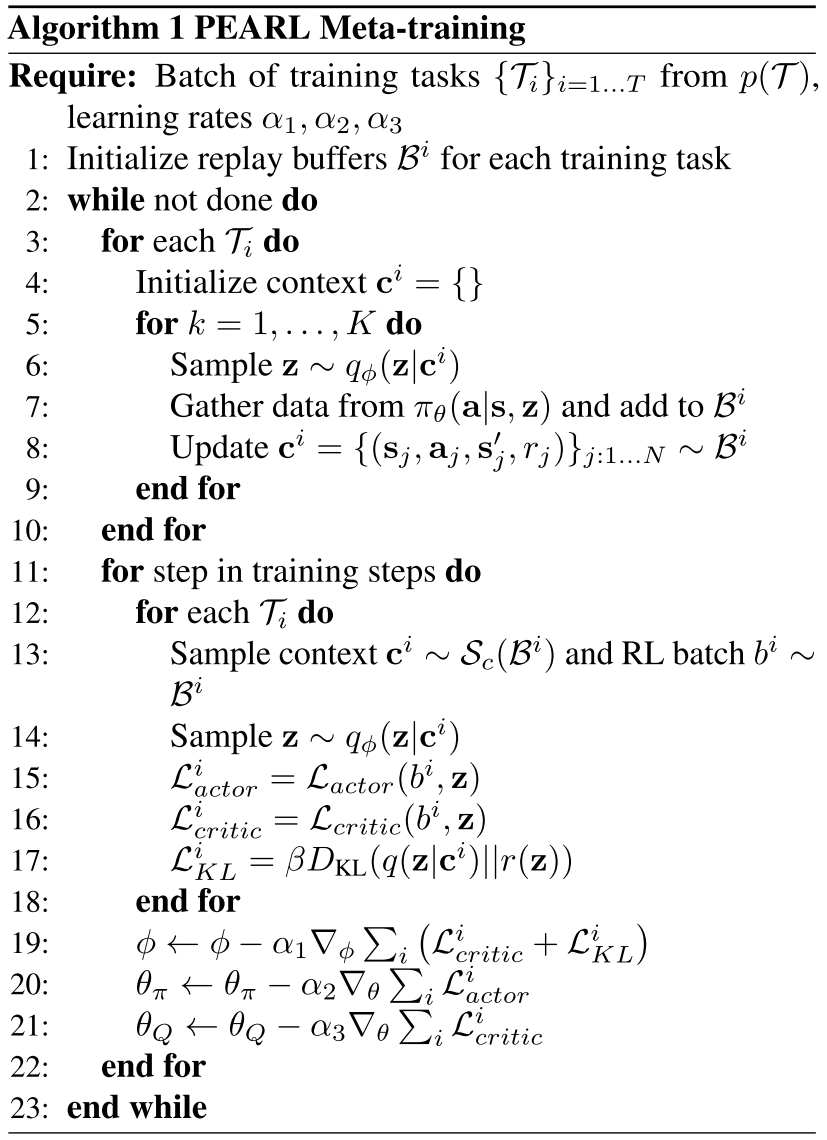
Efficient Off-Policy Meta-Reinforcement Learning via Probabilistic Context Variables

Most current meta-RL methods require on-policy data during both meta-training and adaptation, which makes them exceedingly inefficient during meta-training.

Meta-learning typically operates on the principle that meta-training time should match meta-test time - for example, an image classification meta-learner tested on classifying images from five examples should be meta-trained to take in sets of five examples and produce accurate predictions (Vinyals et al., 2016). This makes it inherently difficult to meta-train a policy to adapt using off-policy data, which is systematically different from the data the policy would see when it explores (on-policy) in a new task at meta-test time.

To achieve both meta-training efficiency and rapid adaptation, we propose an approach that integrates online inference of probabilistic context variables with existing off-policy RL algorithms.

Context-based meta-RL methods.

Probabilistic meta-learning.

Posterior sampling.

Partially observed MDPs.

Problem Statement

Assume a distribution of tasks \(p(T)\), where each task is a Markov decision process (MDP).

Assume that the transition and reward functions are unknown, but can be sampled by taking actions in the environment.

Formally, a task \(T = {p(s_0), p(s_{t+1} | s_t, a_t), r(s_t, a_t)}\), initial state distribution \(p(s_0)\), transition distribution \(p(s_{t+1} | s_t, a_t)\), reward function \(r(s_t, a_t)\).

Given a set of training tasks sampled from \(p(T)\), the meta-training process learns a policy that adapts to the task at hand by conditioning on the history of past transitions, which we refer to as context \(c\).

Let \(c_n^T = (s_n, a_n, r_n, s_n')\) be one transition in the task \(T\) so that \(c_{1:N}^T\) comprises the experience collected so far.

At test-time, the policy must adapt to a new task drawn from \(p(T)\).

Probabilistic Latent Context

We capture knowledge about how the current task should be performed in a latent probabilistic context variable \(Z\), on which we condition the policy as \(\pi_\theta(a | s, z)\) in order to adapt its behavior to the task.

Modeling and Learning Latent Contexts

amortized variational inference

Train an inference network \(q_\phi(z | c)\), that estimates the posterior \(p(z | c)\).

\(q_\phi(z | c)\) can be optimized in a model-free manner to model the state-action value functions or to maximize returns through the policy over the distribution of tasks. Assuming this objective to be a log-likelihood, the resulting variational lower bound is:

$$ \mathbb{E}T[\mathbb{E}{z \sim q_\phi(z | c^T)}[R(T, z) + \beta D_{KL}(q_\phi(z | c^T) || p(z))]] $$

where \(p(z)\) is a unit Gaussian prior over \(Z\) and \(R(T, z)\) could be a variety of objectives, as discussed above.

We note that an encoding of a fully observed MDP should be permutation invariant.

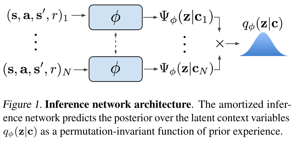
Choose a permutation-invariant representation for \(q_\phi(z | c_{1:N})\), modeling it as a product of independent factors

$$ q_\phi(z | c_{1:N}) \propto \prod_{n=1}^N \Psi_\phi(z | c_n) $$

To keep the method tractable, we use Gaussian factors \(\Psi_\phi(z | c_n) = N(f_\phi^\mu(c_n), f_\phi^\sigma(c_n))\), which result in a Gaussian posterior.

The function \(f_\phi\), represented as a neural network parameterized by \(\phi\), predicts the mean \(\mu\) as well as the variance \(\sigma\) as a function of the \(c_n\), is shown in Figure 1.

Posterior Sampling and Exploration via Latent Contexts

PEARL directly infers a posterior over the latent context Z, which may encode the MDP itself if optimized for reconstruction, optimal behaviors if optimized for the policy, or the value function if optimized for a critic.

Off-Policy Meta-Reinforcement Learning

Our main insight in designing an off-policy meta-RL method with the probabilistic context in Section 4 is that the data used to train the encoder need not be the same as the data used to train the policy.

The policy can treat the context \(z\) as part of the state in an off-policy RL loop, while the stochasticity of the exploration process is provided by the uncertainty in the encoder \(q(z|c)\). The actor and critic are always trained with off-policy data sampled from the entire replay buffer \(B\).

We define a sampler \(S_c\) to sample context batches for training the encoder.

Allowing \(S_c\) to sample from the entire buffer presents too extreme of a distribution mismatch with on-policy test data. However, the context does not need to be strictly on-policy; we find that an in-between strategy of sampling from a replay buffer of recently collected data retains on-policy performance with better efficiency.

soft actor-critic algorithm (SAC), an off-policy actorcritic method based on the maximum entropy RL objective which augments the traditional sum of discounted returns with the entropy of the policy.

The critic loss can then be written as

$$ L_{critic} = \mathbb{E}{(s, a, r, s') \sim B, z \sim q\phi (z | c)} [Q_\theta(s, a, z) - (r + \bar{V}(s', \bar{z}))] ^ 2 $$

where \(\bar{V}\) is a target network and \(\bar{z}\) indicates that gradients are not being computed through it.

The actor loss is nearly identical to SAC, with the additional dependence on \(z\) as a policy input:

$$ L_{actor} = \mathbb{E}{s \sim B, a \sim \pi\theta, z \sim q_\phi(z | c)}[D_{KL}(\pi_\theta(a | s, \bar{z}) \parallel \frac{\exp(Q_\theta(s, a, \bar{z}))}{\mathcal{Z}_\theta(s)})] $$

Autonomous Systems

自动驾驶相关论文。

Planning and Decision-Making for Autonomous Vehicles

1.介绍

主要介绍自动驾驶规划和决策的多个方面，大致分为三种不同的方法：
sequential planning(section 2)，behavior-aware planning(section 4)和end-to-end planning(section 3)。
section 5讲各种方法如何验证和综合，section 6讲自动驾驶车辆车队(fleet)的管理方法。

2.MOTION PLANNING AND CONTROL

主要是一些车辆控制和运动规划的传统方法。
先讲parallel autonomy，再讲autonomous vehicles，最后列出决策和规划目前的一些挑战。

车辆动力学和控制

低速情况下，有运动学模型可以控制车辆。而高速情况下，需要使用车辆的完整动力学模型，包括轮胎的力等。
一些模型：Nonlinear control (18), model predictive control (19), feedback–feedforward control (20)

这些模型依赖于需要识别的车辆模型，有基于优化的技术和基于学习的技术。

parallel autonomy

有三种collaborative autonomy的方式：series autonomy，interleaved autonomy，parallel autonomy。
parallel autonomy指自动驾驶系统处于后台运行来保证安全，而由人来操作车辆，当人被转移注意力或无法处理当前情况时，该系统会提供安全性。

比较直观的做法是将人的输入和安全系统的输出直接线性组合起来，Anderson et al. (23)。

另一种做法是将人的输入以最低影响的方式合并到优化框架中。Alonso-Mora et al. (25)，Shia et al. (26) ，Erlien et al. (27)。

运动规划

大多数计算安全路径的传统方法都是基于以下三种思路：

• 支持碰撞检测的输入空间离散化(input space discretization with collision checking)
  • lattice planners (e.g., 31, 32)
  • road-aligned primitives (e.g., 33)
• 随机规划(randomized planning)
  • rapidly exploring random trees (RRT) (e.g., 34, 35)
• 约束优化和滚动时域控制(constrained optimization and receding-horizon control(e.g., 19, 36))
  • Schwarting et al. (28)

3.INTEGRATED PERCEPTION AND PLANNING

主要介绍感知的前沿技术，描述综合感知和规划的端到端方法(end-to-end methods)，直接从感知信息生成车辆的控制输入，非常依赖机器学习。

从经典感知到基于神经网络的感知系统的目前的挑战

一些benchmarking数据集：KITTI (42), ISPRS (International Society for Photogrammetry and Remote Sensing), MOT (Multiple Object Tracking), and Cityscapes (43)。

经典感知系统从原始感知数据中以人工设计的特征形式提取信息。最著名的一些例子：SIFT (Scale-Invariant Feature Transform) (44, 45), BRISK (Binary Robust Invariant Scalable Keypoints) (46), SURF (Speeded Up Robust Features) (47, 48), and ORB (Oriented FAST and Rotated BRIEF) (49, 50)。
基于纯视觉的迅速、轻量级的方法已经成熟：such asORB-SLAM2 (50), SVO(SemidirectVisualOdometry) 2.0 (52), and LSD-SLAM (Large-Scale DirectMonocular SLAM) (53)。

物体检测一般有两种方式：碰撞盒检测和语义分割。

• 碰撞盒检测
  • the ImageNet Large Scale Visual Recognition Challenge (55)
  • real-time-capable systems such as Faster R-CNN (Faster Regional Convolutional Neural Network) (56)
• 语义分割
  • ResNet38 (57) and PSPNet (Pyramid Scene Parsing Network) (58)
    • achieve more than 80% mIoU (mean intersection over union) in the Cityscapes data set (43)
    • but take multiple seconds to propagate on high-resolution images
  • ENet (Efficient Neural Network) (59)
    • achieved a 13-ms runtime on 1,024×2,048–pixel images with 58% mIoU on theCityscapes data set (43)
  • ICNet (ImageCascadeNetwork) (60)
    • achieved 70% mIoU at 33 ms

真实世界数据集非常昂贵，使用虚拟世界的数据更便宜，训练效果也更好，不过会增加数据集的偏差。

基于神经网络的感知系统有一个很大的问题，不确定性的反馈不足(insufficient feedback of uncertainty)。 网络不确定性可以由Monte Carlo dropout sampling (65)估计。 McAllister et al. (66)提出使用有原则的贝叶斯框架(a principled Bayesian framework)估计和传播整个系统管道中每个组件的不确定性，将使自动驾驶汽车能够适当地应对高不确定性。

端到端规划(End-to-End Planning)

传统的自动驾驶架构中，功能被封装在模块之间清晰可见的接口中，也被称作中介感知(mediated perception)。

另一种架构是对感知模块的某些部分进行训练来包含规划模块的部分任务。

• Caltagirone et al. (68)，通过整合激光雷达点云、GPS-惯性测量单元（IMU）信息和谷歌导航信息来生成行驶路径。
• 语义分割网络可用于在相机图像空间(camera image space (69))中生成路径。

更进一步，架构可以学习车道和道路跟踪的整个任务，而无需手动分解为道路或车道标记检测、语义抽象、路径规划和控制。

• ALVINN (Autonomous Land Vehicle in a Neural Network) (70)，训练神经网络从相机图像输出行驶的转向角，来让车辆保持在道路上行驶。
• Chen et al. (67)将其称为behavior reflex approach。
• NVIDIA (72)，训练了一个深度卷积神经网络，可以将前向摄像头的原始(raw)图像直接映射到转向命令，并能够处理具有挑战性的场景。
• Bojarski et al. (73)，展示了神经网络能够学习类似车道标线、道路边界和其他车辆形状的特征(feature)。
• Xu et al. (75)，使用大规模行驶视频数据集来训练了一个端到端的全卷积LSTM神经网络，可以预测离散行为(直行、停止、左转、右转)和连续行为(方向盘角度控制)。
• SafeDAgger (76)，DAgger (77)。

端到端运动规划也被运用于机器人学。

另一条研究路线是在模拟器中学习驾驶行为，可以在安全环境下观察失败的情况，适合强化学习的训练。

• Wolf et al. (81)，在模拟环境下使用Deep Q-Network来学习驾驶车辆。

4.BEHAVIOR-AWARE MOTION PLANNING

5.VERIFICATION AND SYNTHESIS

6.FLEET MANAGEMENT

A Review of Mobile Robot Motion Planning Methods: from Classical Motion Planning Workflows to Reinforcement Learning-based Architectures

主要分为三个部分：

• CLASSICAL MOTION PLANNING OF MRS
• RL-based motion planning approaches
  • MAP-BASED CLASSICAL MOTION PLANNING ALGORITHMS WITH RL OPTIMIZATION
  • RL-BASED MAPLESS MOTION PLANNING METHODS
  • RL-BASED MULTI-ROBOT MOTION PLANNING
• DISCUSSION

CLASSICAL MOTION PLANNING OF MRS

首先需要获取map representation of the environment，包括occupancy grid map, point cloud map, Voronoi diagram map, Euclidean signed distance fields.

经典运动规划器的经典层次结构如下：

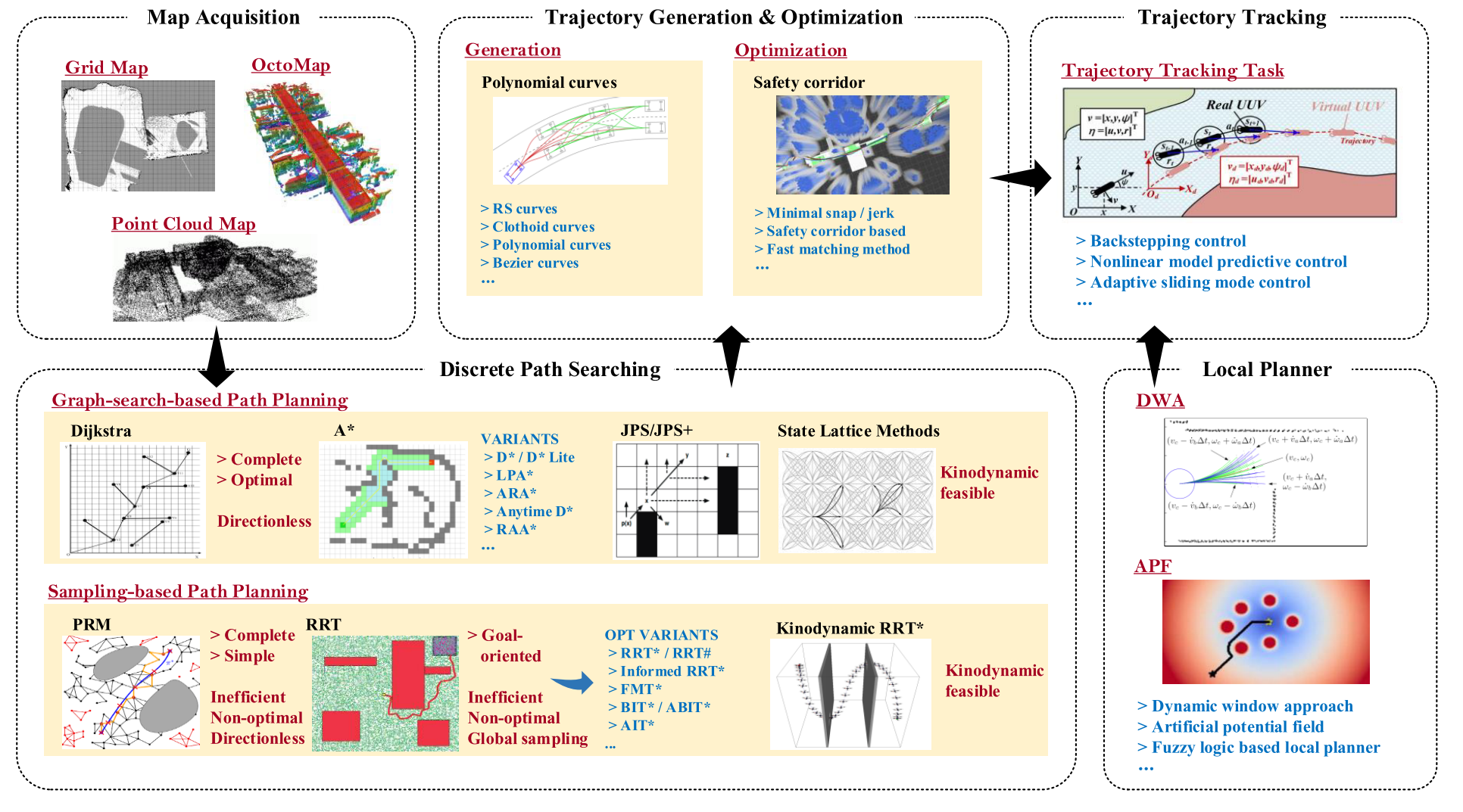
可以分成四个部分：discrete path searching, trajectory generation and optimization, trajectory tracking, and local planner.

discrete path searching

传统全局DPS算法可以分为两类：the graph-searching-based algorithm (GSBA) and the sampling-based algorithm (SBA).

GSBA

主要应用于低维空间上的路径规划问题.

dfs, bfs.

Dijkstra, A*.

Dynamic A* (D*), Lifelong planning A* (LPA*), D* Lite.

Jump point search (JPS), JPS+.

都没考虑运动动力学，State lattice methods被提出来解决这个问题.

SBA

更适合高维空间.

Probabilistic road map (PRM), rapid-exploring random tree (RRT).

RRT*, RRT*-smart, RRT#.

fast match trees (FMT*).

kino-dynamic RRT*, informed RRT*, batch informed trees (BIT*).

Real-time RRT* (RT-RRT*), informationdriven RRT* (ID-RRT*).

trajectory generation and optimization

大多数DPS算法只考虑工作空间的几何约束，在某些情况下，最终的最优或接近最优的分段轨迹对于实际的MR来说是不可执行的.

轨迹生成和优化（TGO）过程考虑了机器人的多重约束（例如，安全约束、运动动力学约束等），并将时间分配机制(time-allocation mechanism)纳入规划过程中，以赋予运动规划器更多的可执行能力。

trajectory generation

interpolation-curve-based method: good continuity and differentiability，典型的包括Reeds and Sheep (RS) curves, clothoid curves, polynomial curves, Bezier curves.

trajectory optimization

minimum snap algorithm.

EDF-based TGO method.

trajectory tracking

使 MR 能够跟踪 TGO 流程规划的轨迹.

local planner

MR需要具备局部重规划能力，以在跟踪全局轨迹的同时应对突发情况.

artificial potential field, reactive replanning method, fuzzy algorithm based method.

其中reactive replanning method 包括 directional approach, dynamic window approach (DWA).

MAP-BASED CLASSICAL MOTION PLANNING ALGORITHMS WITH RL OPTIMIZATION

在上述传统架构中，规划架构的全局规划器和局部规划器是相互独立的，研究人员需要单独开发它们.此外，为了获得最终的可执行轨迹，研究人员必须解决具有多个约束的优化问题. 这个过程增加了规划方法的复杂性. 此外，经典的运动规划器包含各种子模块，每个子模块都需要繁琐的参数调整过程.

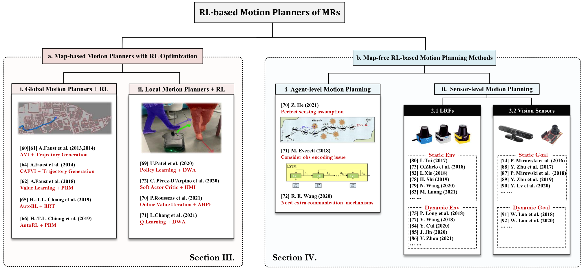
Global Planners Combined with RL Improvements

approximate value iteration (AVI) RL-based motion planning architecture

PRM-RL algorithm, RL-RRT, AutoRL-based PRM-RL.

Local Planners Combined with RL Improvements

目的是让机器人在非结构化、动态和不确定的环境中具有更强的操作能力.

hybrid DWA-RL.

AHPF-RL.

Q-learning-based DWA.

soft actor-critic (SAC)-based local planner.

RL-BASED MAPLESS MOTION PLANNING METHODS

在本节中，我们将审查的重点转移到基于端到端 RL 的运动规划方法，这些运动规划器是无地图的，实现了全局规划器和局部规划器的统一.

可以分为agent-level methods, sensor-level methods两个部分.

agent-level methods

agent-level methods基于预设的状态估计过程，可以直接获取环境的上层状态信息，更容易训练，这使得机器人能够更快地获得最优规划策略. agent-level methods的观测维度较低，包含更多有用信息，其状态可以等效于原始传感器数据的特征提取之后的输出. 更重要的是，agent-level methods的模拟器的开发难度要小得多. 然而，此类方法依赖于完美感知的假设，或者需要考虑观察编码问题，或者需要额外的通信机制来共享状态信息，这些限制限制了agent-level methods的可扩展性和应用.

sensor-level methods

sensor-level methods是端到端的，直接建立从原始传感器数据到规划决策的非线性映射.

根据主流研究趋势，以及常用的机器人感知方法，可以分为laser range finder (LRF) based methods 和 visual-based methods.

Laser Range Finder based

intrinsic curiosity module

D. Pathak, P. Agrawal, A. A. Efros, and T. Darrell, “Curiosity-driven exploration by self-supervised prediction,” in International Conference on Machine Learning. PMLR, 2017, pp. 2778–2787.

H. Shi, L. Shi, M. Xu, and K.-S. Hwang, “End-to-end navigation strategy with deep reinforcement learning for mobile robots,” IEEE Transactions on Industrial Informatics, vol. 16, no. 4, pp. 2393–2402, 2019.

Y. Wang, H. He, and C. Sun, “Learning to navigate through complex dynamic environment with modular deep reinforcement learning,” IEEE Transactions on Games, vol. 10, no. 4, pp. 400–412, 2018.

EWC-DDPG.

上述大多数运动规划器只能部署在数值模拟空间中，sim-to-real problem.

asynchronous DDPG (ADDPG)-based motion planning algorithm.

assisted-DDPG (AsDDPG).

Vision sensors

NavA3C algorithm.

DRL-based targetdriven visual navigation approach.

RL-BASED MULTI-ROBOT MOTION PLANNING

DISCUSSION

Challenges

• Reality Gap
• Sparse reward problem
• Generalization
• Low sample efficiency
• Social etiquette
• Lidar data pre-processing issues
• Catastrophic forgetting problem

Future Directions

• Task-free RL-based general motion planner
• Meta RL-based motion planning methods
• Multi-modal fusion based RL motion planning methods
• Multi-task objectives based RL motion planning methods
• Human-Machine interaction mode based motion planning methods
• RL-based motion planning of multiple heterogeneous MRs
• Multi-MR flexible formation planning methods

RL

Reinforcement learning.

Asynchronous Methods for Deep Reinforcement Learning

Reinforcement Learning Background

Environment \(E\), time step \(t\), state \(s_t\), action \(a_t\), possible actions \(A\), policy \(\pi\), scalar reward \(r_t\).

Return \(R_t = \sum_{k=0}^\infty \gamma^k r_{t+k}, \gamma \in (0, 1]\).

Action value \(Q^\pi(s, a) = \mathbb{E}[R_t | s_t = s, a]\) (expected return).

Optimal action value function \(Q^*(s, a) = \max_\pi Q^\pi(s, a)\).

State value \(V^\pi(s) = \mathbb{E}[R_t | s_t = s] = \sum_{a \in A} \pi(a | s) · Q^\pi(s, a)\).

value-based method (Q-learning)

\(Q(s, a ; \theta) \approx Q^*(s, a)\).

The \(i\)th loss function:

$$ L_i(\theta_i) = \mathbb{E}(r + \gamma \max_{a'} Q(s', a' ; \theta{i-1}) - Q(s, a ; \theta)) ^ 2 $$

where \(s'\) is the state encountered after state \(s\).

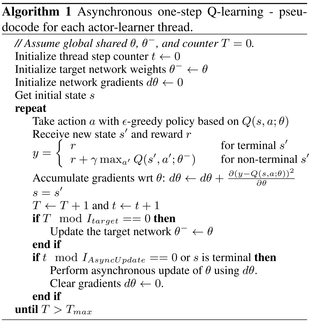
One-step Q-learning.

policy-based methods

\(\pi(a | s ; \theta)\).

Update the parameters \(\theta\) by performing, typically approximate, gradient ascent on \(E[R_t]\).

REINFORCE:

• Updates the policy parameters \(\theta\) in the direction \(\nabla_\theta \log \pi(a_t | s_t ; \theta) R_t\) which is an unbiased estimate of \(\nabla_\theta \mathbb{E} [R_t]\).
• Reduce the variance of this estimate while keeping it unbiased by subtracting a learned function of the state \(b_t(s_t)\), known as a baseline (Williams, 1992), from the return. Resulting gradient: \(\nabla_\theta \log \pi(a_t | s_t ; \theta) (R_t - b_t(s_t))\).

Actor-critic:

• A learned estimate of the value function is commonly used as the baseline \(b_t(s_t) \approx V^\pi(s_t)\) leading to a much lower variance estimate of the policy gradient.
• The quantity \(R_t − b_t\) used to scale the policy gradient can be seen as an estimate of the advantage of action at in state \(s_t\), or \(A(a_t, s_t) = Q(a_t, s_t)−V(s_t)\).

Asynchronous RL Framework

First, asynchronous actor-learners, multiple CPU threads on a single machine.

Second, make the observation that multiple actors-learners running in parallel are likely to be exploring different parts of the environment, use different exploration policies in each actor-learner to maximize this diversity.

Benefits:

• Stabilizing learning: By running different exploration policies in different threads, the overall changes being made to the parameters by multiple actor-learners applying online updates in parallel are likely to be less correlated in time than a single agent applying online updates.
• Reduction in training time that is roughly linear in the number of parallel actor-learners.
• Able to use on-policy reinforcement learning methods such as Sarsa and actor-critic to train neural networks in a stable way.

Asynchronous onestep Q-learning

Asynchronous one-step Sarsa

Same as asynchronous one-step Q-learning except that it uses a different target value for \(Q(s, a)\) : \(r + \gamma Q(s', a' ; \theta^-)\).

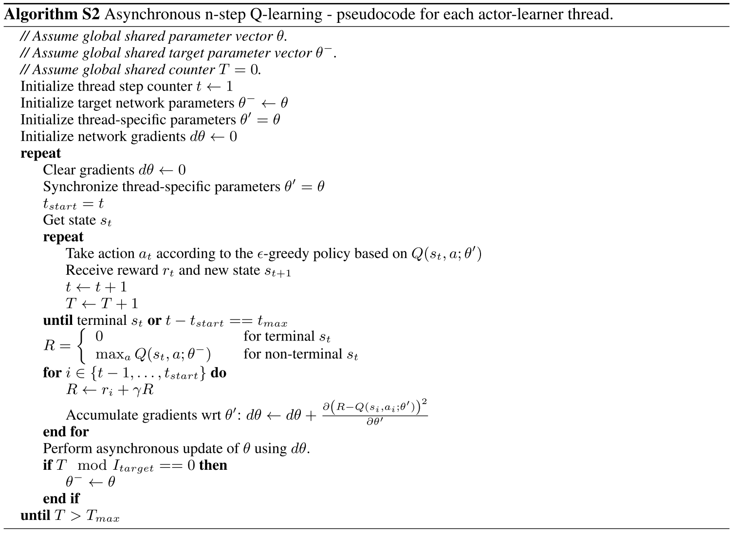
Asynchronous n-step Q-learning

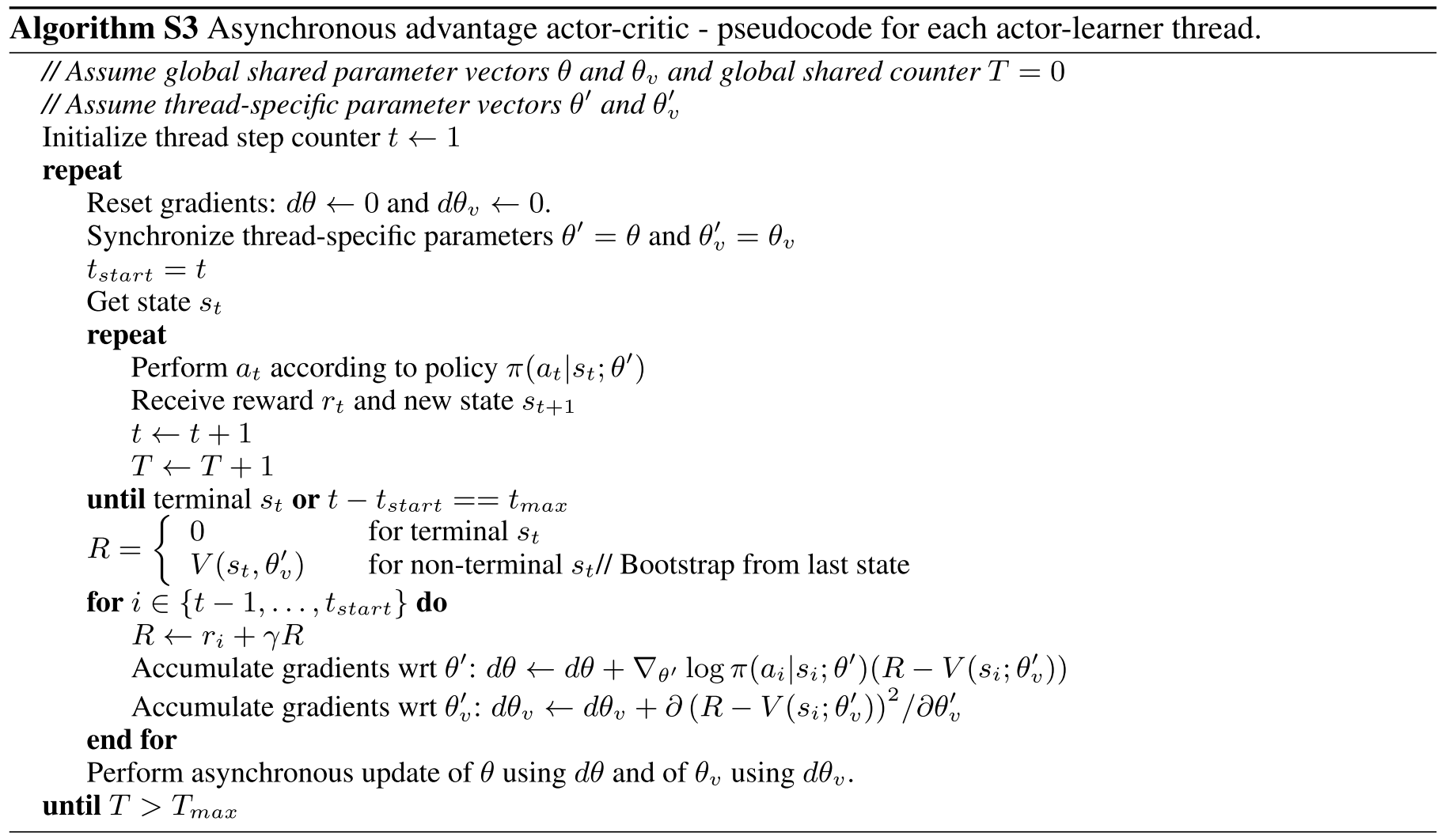
Asynchronous advantage actor-critic (A3C)

A3C maintains a policy \(\pi(a_t|s_t; \theta)\) and an estimate of the value function \(V(s_t; \theta_v)\).

Like the variant of n-step Q-learning, the variant of actor-critic also operates in the forward view and uses the same mix of n-step returns to update both the policy and the value-function.

LEARNING TO NAVIGATE IN COMPLEX ENVIRONMENTS

APPROACH

An end-to-end learning framework that incorporates multiple objectives:

• maximize cumulative reward using an actor-critic approach.
• minimizes an auxiliary loss of inferring the depth map from the RGB observation.
• detect loop closures as an additional auxiliary task that encourages implicit velocity integration.

The reinforcement learning problem is addressed with the Asynchronous Advantage Actor-Critic (A3C) algorithm.

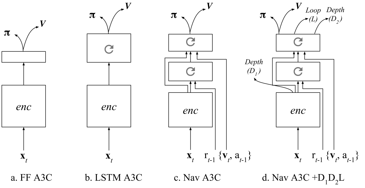
The baseline: an A3C agent that receives only RGB input from the environment, using either a recurrent or a purely feed-forward model (Figure 1a,b).

To support the navigation capability of our approach, we also rely on the Nav A3C agent (Figure 1c) which employs a two-layer stacked LSTM after the convolutional encoder.

Image \(\bf{x}t \in \mathbb{R}^{3 \times W \times H}\), the agent-relative lateral and rotational velocity \(\bf{v} \in \mathbb{R}^6\), the previous action \(a{t-1} \in \mathbb{R}^{N_A}\), and the previous reward \(r_{t-1} \in \mathbb{R}\).

Figure 1d shows the augmentation of the Nav A3C with the different possible auxiliary losses.

DEPTH PREDICTION

While depth could be directly used as an input, we argue that if presented as an additional loss it is actually more valuable to the learning process.

Since the role of the auxiliary loss is just to build up the representation of the model, we do not necessarily care about the specific performance obtained or nature of the prediction. We do care about the data efficiency aspect of the problem and also computational complexity. We use a low resolution variant of the depth map, reducing the screen resolution to 4x16 pixels.

Two different variants for the loss:

• A regression task. While this formulation, combined with a higher depth resolution, extracts the most information, mean square error imposes a unimodal distribution.
• A classification loss, where depth at each position is discretised into 8 different bands. While it greatly reduces the resolution of depth, it is more flexible from a learning perspective and can result in faster convergence (hence faster bootstrapping).

LOOP CLOSURE PREDICTION

To produce the training targets, we detect loop closures based on the similarity of local position information during an episode, which is obtained by integrating 2D velocity over time.

Curiosity-driven Exploration by Self-supervised Prediction

In many real-world scenarios, rewards extrinsic to the agent are extremely sparse or missing altogether, and it is not possible to construct a shaped reward function.

In reinforcement learning, intrinsic motivation/rewards become critical whenever extrinsic rewards are sparse.

Two broad classes:

• encourage the agent to explore “novel” states
• encourage the agent to perform actions that reduce the error/uncertainty in the agent’s ability to predict the consequence of its own actions

The effectiveness of curiosity formulation in all three of these roles:

• solving tasks with sparse rewards
• helps an agent explore its environment in the quest for new knowledge
• learn skills that might be helpful in future scenarios

Curiosity-Driven Exploration

Intrinsic curiosity reward generated by the agent at time t: \(r_t^i\), extrinsic reward: \(r_t^e\), sum: \(r_t = r_t^i + r_t^e\), with \(r_t^e\) mostly zero.

Policy: \(\pi(s_t ; \theta_P)\) by a deep neural network with parameters \(\theta_P\).

Given the agent in state \(s_t\), it executes the action \(a_t \sim \pi(s_t ; \theta_P)\).

\(\theta_P\) is optimized to maximize the expected sum of rewards:

$$ \max_{\theta_P} \mathbb{E}_{\pi(s_t ; \theta_P)} [\Sigma_t r_t] $$

Asynchronous advantage actor critic policy gradient (A3C).

Prediction error as curiosity reward

If not the raw observation space, then what is the right feature space for making predictions so that the prediction error provides a good measure of curiosity?

Divide all sources that can modify the agent’s observations into three cases:

• things that can be controlled by the agent;
• things that the agent cannot control but that can affect the agent (e.g. a vehicle driven by another agent), and
• things out of the agent’s control and not affecting the agent (e.g. moving leaves).

A good feature space for curiosity should model (1) and (2) and be unaffected by (3).

Self-supervised prediction for exploration

A general mechanism for learning feature representations such that the prediction error in the learned feature space provides a good intrinsic reward signal.

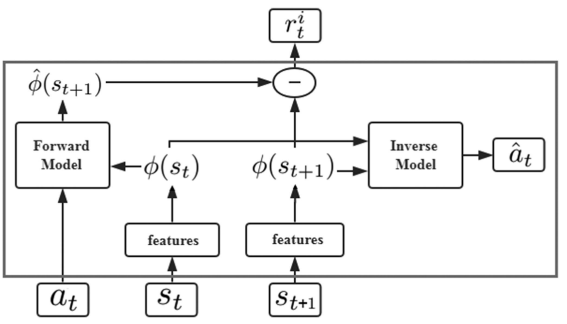
Train a deep neural network with two sub-modules:

• the first submodule encodes the raw state \((s_t)\) into a feature vector \(\phi(s_t)\).
• the second submodule takes as inputs the feature encoding \(\phi(s_t), \phi(s_{t+1})\) of two consequent states and predicts the action \((a_t)\) taken by the agent to move from state \(s_t\) to \(s_{t+1}\).

Training this neural network amounts to learning function \(g\) defined as:

$$ \hat{a}t = g(s_t, s{t+1} ; \theta_I) $$

The neural network parameters \(\theta_I\) are trained to optimize:

$$ \min_{\theta_I} L_I(\hat{a}t, a_t) $$ The learned function \(g\) is also known as the inverse dynamics model and the tuple \((s_t, a_t, s{t+1})\) required to learn \(g\) is obtained while the agent interacts with the environment using its current policy \(\pi(s)\).

Train another neural network:

$$ \hat{\phi}(s_{t+1}) = f(\phi(s_t), a_t ; \theta_F) $$

The neural network parameters \(\theta_F\) are optimized by minimizing the loss function \(L_F\):

$$ L_F(\phi(s_t), \hat{\phi}(s_{t+1})) = \frac{1}{2} \parallel \hat{\phi}(s_{t+1}) - \phi(s_{t+1}) \parallel _2^2 $$

The learned function \(f\) is also known as the forward dynamics model.

The intrinsic reward signal is computed as:

$$ r_t^i = \frac{\eta}{2} \parallel \hat{\phi}(s_{t+1}) - \phi(s_{t+1}) \parallel _2^2 $$

Intrinsic Curiosity Module (ICM).

The overall optimization problem:

$$ \min_{\theta_P, \theta_I, \theta_F} [-\lambda \mathbb{E}_{\pi(s_t;\theta_P)}[\Sigma_t r_t] + (1-\beta) L_I + \beta L_F], 0 \leq \beta \leq 1, \lambda > 0. $$

End-to-End Navigation Strategy With Deep Reinforcement Learning for Mobile Robots

Problem Statement

Navigation strategies for mobile robots in a map-less environment.

A motion planning model based on DRL. This end-to-end model transfers directly the inputs of the sensor observations and the relative position of the target to the commands of robot’s movement.

Uses intrinsic curiosity to allow agents to explore the environment more effectively and as an additional reward in an environment where the rewards are sparse. Sparse laser ranging results are also used as the highly abstracted inputs, so agent strategies that are learned by the simulation are effective in the real world.

Curiosity-Driven Exploration

The original states \((s_t,s_{t+1})\) are encoded into the corresponding features \((\phi(s_t), \phi(s_{t+1}))\).

The inverse model is trained to predict at using state features \((\phi(s_t),\phi(s_{t+1}))\).

\(a_t\) and \(\phi(s_t)\) are passed to the forward model, which is used to predict the feature representation \(\phi(s_{t+1})\) for the state \((s_{t+1})\) and compare it with the real feature \((\phi(s_t))\).

For the inverse model, the goal is to learn the function \(g\) as follows:

$$ \hat{a}t = g(s_t, s{t+1} ; \theta_I) $$

where \(\hat{a}_t\) is the predicted value of the agent’s action \((a_t)\) and \(\theta_I\) is the neural network parameter that is trained to be optimized as follows:

$$ \min_{\theta_I} L_I(\hat{a}_t, a_t) $$

Since the action space is discrete, the output of \(g\) is a soft-max distribution across all possible actions.

The loss function \(L_I\) is set in the form of cross entropy as follows:

$$ L_I(\hat{a}t, a_t) = \sum{i=1}^n -P(a_{t_i}) \ln q(\hat{a}_{t_i}) $$

where \(n\) is the size of the action space, \(P(a_{t_i})\) is whether the agent chooses the \(i\)th action in the actual situation, and \(q(\hat{a}_{t_i})\) is the probability of the agent choosing the \(i\)th action in the prediction result.

Another neural network is trained for the forward model:

$$ \hat{\phi}(s_{t+1}) = f(\phi(s_t), a_t, \theta_F) $$

The training process is performed by minimizing the loss function LF as follows:

$$ L_F(\phi(s_t), \hat{\phi}(s_{t+1})) = \frac{1}{2} \parallel \hat{\phi}(s_{t+1}) - \phi(s_{t+1}) \parallel _2^2 $$

The intrinsic reward signal \(r_t^i\) measured by the prediction error of the feature encoding is calculated as:

$$ r_t^i = \frac{\eta}{2} \parallel \hat{\phi}(s_{t+1}) - \phi(s_{t+1}) \parallel _2^2 $$

where \(\eta > 0\) is the scale factor used to adjust the intrinsic reward.

Navigation Strategy Based on DRL

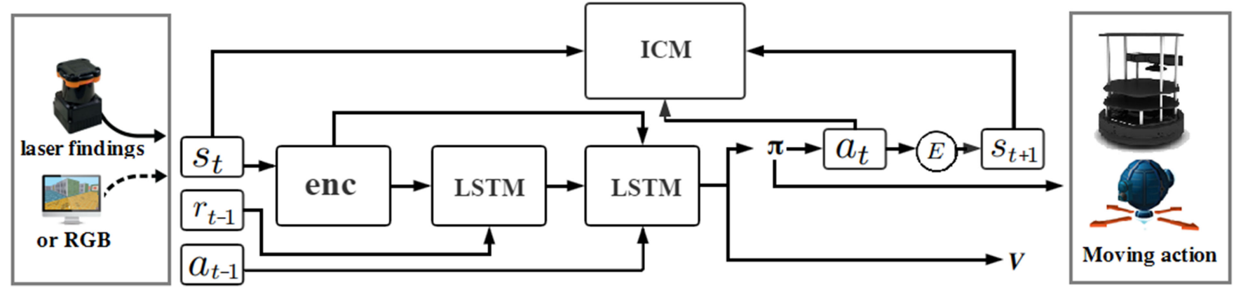
The first layer of LSTM accepts the previous rewards and observations. The aim is to establish an association between the original observations and rewards and transmit this to the next level of LSTM. The previous action is passed directly to the LSTM of the second layer.

Finally, connected to two separate output layers including softmax layer and linear layer, respectively, generating policy \(\pi\) and value function \(V\).

The reward function is divided into two components: the agent interacting with the environment obtains the extrinsic reward \(r_t^e\) and the intrinsic reward \(r_t^i\).

The policy \(\pi(s_t ; \theta_p)\) is represented by a deep neural network with the parameter \(\theta_p\).

Sum of the intrinsic reward: \(r_t = r_t^e + r_t^i\).

The problem that needs to be optimized overall:

$$ \min_{\theta_p, \theta_I, \theta_F} \Big [-\lambda \mathbb{E}_{\pi(s_t ; \theta_p)}\big [ \sum_t r_t \big ] + (1-\beta) L_I + \beta L_F \Big ] $$

where \(\lambda > 0\) is used to adjust the weight of the policy gradient loss for the curiosity reward, and \(0 \leq \beta \leq 1\) is used to adjust the weight between the forward model loss and the inverse model loss.

LEARNING TO NAVIGATE IN COMPLEX ENVIRONMENTS

APPROACH

An end-to-end learning framework that incorporates multiple objectives:

• maximize cumulative reward using an actor-critic approach.
• minimizes an auxiliary loss of inferring the depth map from the RGB observation.
• detect loop closures as an additional auxiliary task that encourages implicit velocity integration.

The reinforcement learning problem is addressed with the Asynchronous Advantage Actor-Critic (A3C) algorithm.

The baseline: an A3C agent that receives only RGB input from the environment, using either a recurrent or a purely feed-forward model (Figure 1a,b).

To support the navigation capability of our approach, we also rely on the Nav A3C agent (Figure 1c) which employs a two-layer stacked LSTM after the convolutional encoder.

Image \(\bf{x}t \in \mathbb{R}^{3 \times W \times H}\), the agent-relative lateral and rotational velocity \(\bf{v} \in \mathbb{R}^6\), the previous action \(a{t-1} \in \mathbb{R}^{N_A}\), and the previous reward \(r_{t-1} \in \mathbb{R}\).

Figure 1d shows the augmentation of the Nav A3C with the different possible auxiliary losses.

DEPTH PREDICTION

While depth could be directly used as an input, we argue that if presented as an additional loss it is actually more valuable to the learning process.

Since the role of the auxiliary loss is just to build up the representation of the model, we do not necessarily care about the specific performance obtained or nature of the prediction. We do care about the data efficiency aspect of the problem and also computational complexity. We use a low resolution variant of the depth map, reducing the screen resolution to 4x16 pixels.

Two different variants for the loss:

• A regression task. While this formulation, combined with a higher depth resolution, extracts the most information, mean square error imposes a unimodal distribution.
• A classification loss, where depth at each position is discretised into 8 different bands. While it greatly reduces the resolution of depth, it is more flexible from a learning perspective and can result in faster convergence (hence faster bootstrapping).

LOOP CLOSURE PREDICTION

To produce the training targets, we detect loop closures based on the similarity of local position information during an episode, which is obtained by integrating 2D velocity over time.

Learning to Navigate Through Complex Dynamic Environment With Modular Deep Reinforcement Learning

Main contributions:

• A modular architecture for navigation problems is proposed to separately resolve local obstacle avoidance and global navigation, which enables modularized training and promotes generalization ability.
• A novel two-stream Q-network is developed for obstacle avoidance. By separating spatial and temporal information from raw input and processing them individually, this new approach supplements temporal integration of agent observations and surpasses the conventional DQL approach in moving obstacle avoidance tasks.
• We proposed an action scheduling method, which combines and exploits the pretrained policies for efficient exploration and online learning in unknown environments.

RELATED WORK

Traditional Robotics

The Potential Field Method (PFM).

Vector field histogram (VFH), VFH+, VFH*.

Simultaneous localization and mapping (SLAM), vision-based SLAM.

Reinforcement Learning

Hierarchical reinforcement learning.

The option framework, concurrent option framework, HAM, MAXQ.

DRL: Double Qlearning, Dueling network architecture, deep deterministic policy gradient method, A3C, Hierarchical-DQN.

PROPOSED APPROACHES

Divide and conquer strategy, divide the main navigation task into two subtasks: local avoidance and global navigation.

Avoidance Module

The simulated environment is formalized as a Markov Decision Process (MDP) described by a 4-tuple \(S, A, P, R\).

Time step \(t\), state \(s_t \in S\), action \(a_t \in A \), policy \(\pi\), reward \(r_t \sim R(s_t, a_t)\), new state \(s_{t+1} = P(s_t, a_t)\), return \(R_t = \sum_{t'=t}^T \gamma^{t'-t} r_t', \gamma \in [0, 1]\).

Action-value function or Q-function: \(Q^\pi(s, a) = \mathbb{E}[R_t | s_t=s, a_t=a]\).

Optimal Action-value function or optimal Q-function: \(Q^*(s, a) = \max_\pi \mathbb{E}[R_t | s_t=s, a_t=a]\).

This optimal action-value function verifies the Bellman optimality equation: \(Q^(s, a) = \mathbb{E}[r + \gamma \max_{a'} Q^(s', a') | s, a]\).

Then, the Q-function can be estimated by utilizing this equation as an iterative update, which is given by

$$ Q(s, a) \leftarrow Q(s, a) + \alpha [r + \gamma \max_{a'} Q(s', a') - Q(s, a)]. $$

For this avoidance task with LRF observations in a dynamic environment, we proposed a two-stream Q-network to approximate the action-value function.

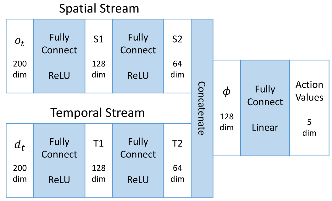
The spatial part is the raw laser scan \(o_t\); the temporal part is the difference between the present and the previous laser scans, namely, \(d_t = o_t - o_{t-1}\).

The two-stream Q-network is present as \(Q^\theta (s_t, a_t), s_t = (o_t, d_t)\).

Two main techniques are employed:

• experience replay
  • The agent’s transition experience \(e = (s_t, a_t, r_t, s_{t+1})\) of each step is stored in a replay buffer \(D = (e_1, \dots, e_N)\).
• double Q-learning
  • A separated network termed target network is introduced to estimate the target for gradient descent update of the main network.

The weights of the main network at training iteration i are updated by minimizing the loss function:

$$ L_i(\theta_i) = \mathbb{E}_{e \sim D} [(y_i - Q^{\theta_i}(s_t, a_t))^2] $$

$$ y_i = r + \gamma \hat{Q}^{\theta^-}(s_{t+1}, \argmax_{a'} Q^{\theta_i}(s_{t+1}, a')) $$

\(y_i\) is the updating target from the separated target network \(\hat{Q}\) with parameters\(\theta^-\).

The update is performed by gradient descent:

$$ \nabla_{\theta_i}L_i(\theta_i) = \mathbb{E}{e \sim D} [(y_i - Q^{\theta_i}(s_t, a_t)) \nabla{\theta_i} Q^{\theta_i}(s_t, a_t)] $$

$$ \theta_{i+1} \leftarrow \theta_i - \alpha \nabla_{\theta_i}L_i(\theta_i) $$

The learned avoidance control policy: \(\pi^\theta(s) = \argmax_a Q^\theta(s, a)\).

To ensure continual exploration, the action is selected by an \(\epsilon\)-greedy strategy.

Navigation Module

Two parts:

• the offline part
  • solve the simple navigation subtask: seeking the fastest policy to drive the agent directly to the destination only based on the relative coordinates in a blank environment without any moving obstacles.
  • standard Q-learning algorithm: input is the 2-D vector \(p_t\), a large positive reward for reaching the destination and a small negative reward for every time step to urge the agent to get the destination in the fastest way.
• the online part
  • two inputs: 1) a 2-D relative coordinates vector of the destination \(p_t\); 2) a 128-D feature \(\phi\) from the avoidance module, which conveys both spatial and temporal information of the surrounding situation.
  • a positive reward for reaching the destination and a negative reward for collision and also a small time punishment in each step.
  • the training procedure follows the DQL algorithm, experience replay and double Q-learning.
  • an action scheduler to pick up the actions from three action alternatives.

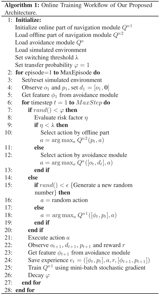
Action Scheduler

The real-time risk factor \(\eta\) is defined as

$$ \eta = \frac{1}{\min(o_t - \kappa d_t)}, \kappa \in [0, 1] $$

switching threshold \(\lambda\), the switching strategy:

$$ a = \begin{cases} action_{n2} \ \ \eta < \lambda \ action_a \ \ \eta \geq \lambda \ \end{cases} $$

where action_a and action_n2 are the action alternatives offered by the avoidance module and the offline part of the navigation module, respectively.

To guarantee a smooth transfer, we introduce a self-decaying transfer probability \(\varphi\). In each step, the agent follows the heuristic policy with the probability \(\varphi\) for heuristic exploration, with probability \((1-\varphi)(1-\epsilon)\) to exploit its online learning policy.

Besides, we still keep a small probability \(\epsilon\) for random exploration to further promote the performance. The (\varphi\) starts from 1 and decays in each step utill 0.